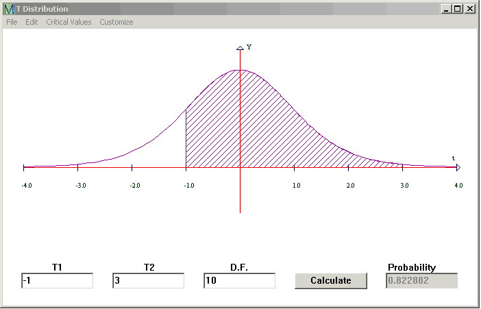
Student's t Distribution is commonly used if you are working with the average of a small number of data. It works much like the Normal Distribution and its graph is also a bell curve. The bell is more spread out though, and the smaller the Degrees of Freedom the more it spreads out.
CalGraph will calculate the chance under the bell curve, that is, the probability that the t variable lies between two values.
Click on Statistics at the top of the window and then on T Distribution. This window opens.

Type the lower number in the first box, the higher number in the second box and the number of Degrees of Freedom in the DF box. Then click Calculate.
Here CalGraph shows that the chance the Student's t variable with 10 Degrees of Freedom is between -1 and 3 is 0.822992. The graph shows the area under the curve shaded.
You may want the area below some value, say t < -2, which means minus infinity < t < -2. Because the curve is close to the axis, you can put -100 (or any number below -100) in the left box. To six decimal places there is no difference in the area. (Okay, I lied to you. For very low degrees of freedom, like DF = 1 or 2, it will make a small difference to the probability.)
Again, you might want the area above some value, maybe t > 3 This means 3 < t < infinity. Put 100 (or any number above 100) in the second box. Don't forget to type in the Degrees of Freedom.
You can print the graph and your result by clicking File and then Print. Or you can copy it to another document, using Edit > Copy Graph to Clipboard and then Paste in that document.
CalGraph will also calculate the other way,
Given an area, CalGraph will find the t-value which cuts off that area. At the top of the T Distribution window, click on Critical Values and then Alpha.
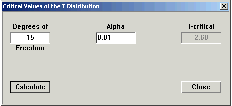
Type in the Degrees of Freedom. Type the area you know in the alpha box and click Calculate.
Here using 15 Degrees of Freedom, 0.01 is the area of the region under the curve between 2.60 and infinity.
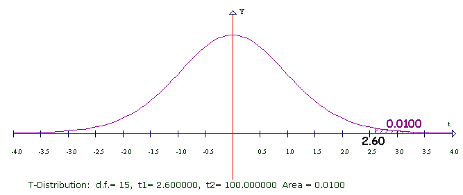
I added some numbers to the graph. I hope this makes the idea clear.
You may want a probability bigger than 50% = 0.5
The T Distribution graph is symmetric. The vertical line cuts the bell in half, 0.5 on each side. So the t you want will be negative. To get this value, put one minus the area you want in the Alpha box, and make the answer negative.
Here's one done out: I wanted 0.9 to be the area under the curve.
1 - 0.9 = 0.1 so I put .1 in the Alpha box.
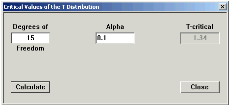
Now I make the T negative: the critical value of T = -1.34 Here's the graph of what happened.
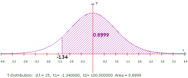
You can see the area is not exactly 0.9. This is round-off error.
CalGraph will calculate the p-value for a hypothesis test.